Poker math gives precise answers to conditional questions. Good decisions also require knowing which conditions you have assumed.
An advanced research essay on no-limit Texas hold’em, with fictional worked models, static equations and downloadable calculations. Read it in sections using the outline. This is an educational synthesis, not a peer-reviewed research paper or a report of my results.
New to poker? Begin with the rules and complete-hand guide or the short foundation lessons. For a quick calculation, use the math reference. This essay is optional deeper reading, not a prerequisite for the beginner checkpoint.
Notation: bb = big blinds; EV = expected value; equity = expected share of the pot at showdown under specified cards and ranges. A = ace, K = king, Q = queen, J = jack and T = ten; ♠, ♥, ♦ and ♣ are suits. AJs means ace-jack of the same suit. Decimal range weights are assumed relative frequencies per legal combination, not measured player statistics. All hand examples omit rake unless stated.
What the numbers can tell you
Abstract. No-limit Texas hold'em is not merely a game in which probabilities are calculated. It is a sequential decision problem in which some uncertainty is generated by random cards, some by hidden information, some by strategic opponents, and some by uncertainty in the player's own model. This distinction is central. Deck probabilities can often be calculated exactly; opponent ranges usually must be inferred; future strategic responses require game-theoretic modeling; and observed profits are noisy statistical evidence rather than direct measurements of decision quality.
This article develops a unified framework joining combinatorics, conditional probability, Bayesian inference, expected-value analysis, statistical estimation, game theory, simulation, tournament equity, bankroll risk, and cognitive science. It draws on foundational work in games of incomplete information, modern computational-poker research, empirical studies of poker performance, and established statistical methodology. Counterfactual regret minimization, DeepStack, Libratus, and Pluribus demonstrate how sophisticated imperfect-information reasoning can be operationalized computationally, while large observational poker datasets show that performance contains persistent skill signals without eliminating substantial short-run randomness. (Harsanyi 1967; Zinkevich et al. 2007; Moravčík et al. 2017; Brown & Sandholm 2018; Brown & Sandholm 2019; Potter van Loon et al. 2015)
The central conclusion is that statistically mature poker reasoning separates known chance probabilities, estimated hidden-state probabilities, strategic response models, and sampling uncertainty. A precise equity calculation can be strategically useless if the range is wrong. A profitable month can be weak evidence of long-run edge. A solver can approximate equilibrium accurately inside its model while giving false confidence when the real opponent lies outside that model. The best statistical process is therefore iterative: condition on known cards, construct and update ranges, calculate action values, test sensitivity to uncertain assumptions, choose the action appropriate to the objective, and update the model as new information arrives.
Central thesis. Poker presents at least three distinct forms of uncertainty:
- Aleatory uncertainty: randomness in which unseen cards are dealt.
- Epistemic and behavioral uncertainty: uncertainty about an opponent's private cards and strategy.
- Model uncertainty: uncertainty about whether one's range, likelihood, equilibrium, variance, or population model is itself appropriate.
This taxonomy is a synthesis, not a claim that poker research has standardized those exact labels. It explains why “knowing the odds” is necessary but radically insufficient. Harsanyi's formal treatment of games with incomplete information made probability distributions over hidden types part of strategic analysis; modern poker algorithms similarly operate over information sets and distributions rather than pretending the hidden state is known. (Harsanyi 1967; Harsanyi 1968; Zinkevich et al. 2007)
Probability asks questions such as, “Given these known cards, what fraction of legal rivers complete a flush?” Statistical inference asks, “Given the opponent's past behavior and present action, what should I believe about their range?” Decision theory asks, “Given those beliefs and consequences, which action has the highest expected objective?” Game theory asks, “How do optimal choices change when the opponent deliberately adapts?” These are connected disciplines, but they are not interchangeable.
The distinction between expectation and realization is equally important. Expected value is an average over hypothetical repetitions under a specified probabilistic model. The payoff from one actual hand is one draw from that distribution. Consequently, a correct call can lose and an incorrect call can win without contradiction. Empirical studies support persistent skill differences in poker, but they also illustrate the danger of translating a population-level result into a universal personal sample-size rule. Levitt and Miles found that players identified as highly skilled before the 2010 WSOP produced much higher tournament ROI than the comparison group, while Potter van Loon and colleagues found performance persistence in an enormous online cash-game dataset. Their conclusions support a role for skill; neither study can certify the true win rate of an arbitrary player today. (Levitt & Miles 2014; Potter van Loon et al. 2015)
Read the research in context
| Source | Year | Methods | Sample size | Key findings | Limitations |
|---|---|---|---|---|---|
| Zinkevich et al., CFR | 2007 | Counterfactual regret minimization in extensive-form imperfect-information games | Poker abstractions up to states | Counterfactual regret minimization can drive self-play toward Nash equilibrium in two-player zero-sum settings | Demonstrated on abstractions; equilibrium guarantees do not automatically transfer to arbitrary multiplayer poker |
| Lanctot et al., MCCFR | 2009 | Sampled CFR using outcome/external sampling | Computational game experiments | Unbiased sampled updates can greatly lower per-iteration computational cost | Sampling introduces variance and convergence trade-offs |
| Bowling et al., Cepheus | 2015 | CFR-family computation for heads-up limit hold'em | Full strategic computation rather than human trial | Heads-up limit hold'em was essentially weakly solved under the paper's criterion | Limit hold'em differs profoundly from no-limit multiplayer play |
| Potter van Loon et al. | 2015 | Observational cash-game data, persistence regressions, simulations | 76.9 million hands, 456.1 million player-hand observations, over 600,000 accounts | Earlier performance predicted later performance; modeled skill signal increases with sample size | Historical mined data, nonrandom player selection, site/stakes/time specificity, serial-dependence concerns |
| Moravčík et al., DeepStack | 2017 | Recursive decomposition, learned value function, continual resolving | About 44,000 professional-play hands | Statistically significant expert-level HUNL performance | Human-match evidence plus an approximate game model, not proof of universal optimality |
| Brown & Sandholm, Libratus | 2018 | Blueprint strategy, nested subgame solving, self-improvement | 120,000 hands against four top HUNL specialists | Defeated the professional group | Heads-up zero-sum setting; human sample small even though hand count was large |
| Burch et al., AIVAT | 2018 | Unbiased control-variate style variance reduction | Poker agent evaluations | Reported 85% SD reduction in a HUNL human-machine match, implying far fewer hands for comparable inference | Requires appropriate known-strategy/value information; not a generic estimator for ordinary player databases |
| Brown & Sandholm, Pluribus | 2019 | Self-play blueprint plus real-time search in six-player NLHE | 10,000-hand principal human experiment | Outperformed elite human professionals; reported adjusted mean of 47.7 mbb/game, SE 25 | Multiplayer games lack the same equilibrium guarantees available in two-player zero-sum games |
| Harville | 1973 | Sequential finish-order probabilities from win probabilities | 335 horse races | Mathematical structure later useful for rank-order models such as poker ICM | Not originally a poker model; ICM inherits strong behavioral simplifications |
The CFR and MCCFR descriptions are supported by the original NeurIPS publications. HUNL means heads-up no-limit hold’em; NLHE means no-limit hold’em; mbb/game means thousandths of a big blind per hand. In Pluribus’s principal five-humans-plus-one-AI experiment, the supplement reports 47.7 mbb/game with standard error 25 and p = .028. A two-sided normal 95% interval using those rounded values includes zero. The relation to a one-sided normal profit test is an explanatory calculation, not a claim that a two-sided 95% interval excludes zero. The experiments establish results in their tested settings, not a guarantee for other players or games. (Zinkevich et al. 2007; Lanctot et al. 2009) DeepStack, Libratus, Pluribus, AIVAT, and the observational poker studies provide complementary forms of evidence rather than interchangeable proof. (Moravčík et al. 2017; Brown & Sandholm 2018; Brown & Sandholm 2019; Burch et al. 2018; Potter van Loon et al. 2015)
A useful historical trajectory is therefore:
The practical lesson of this history is not that humans should imitate an AI's numerical output. It is that successful poker analysis progressively replaced point guesses with distributions over hidden states, and replaced isolated equity calculations with sequential strategic optimization. (Zinkevich et al. 2007; Moravčík et al. 2017; Brown & Sandholm 2018; Brown & Sandholm 2019)
Count cards and calculate equity
The combinatorial foundation. A standard deck has 52 distinct cards. A two-card hold'em hand is an unordered selection, so the number of possible private holdings is
The familiar “169 starting hands” representation collapses suit detail. There are 13 pocket-pair categories, suited nonpair rank categories, and 78 offsuit categories:
But these classes are not equally numerous. Each pocket pair has
physical combinations. Each suited nonpair hand has 4, and each offsuit nonpair hand has .
Worked example: what the 169-grid conceals. Across all rank categories,
Thus, treating each of the 169 labels as equally likely is mathematically wrong. An offsuit category contains twice as many combinations as a pocket pair and three times as many as its suited counterpart.
| Starting-hand class | Rank categories | Combos per category | Physical combos | Share of 1,326 |
|---|---|---|---|---|
| Pocket pairs | 13 | 6 | 78 | 5.88% |
| Suited nonpairs | 78 | 4 | 312 | 23.53% |
| Offsuit nonpairs | 78 | 12 | 936 | 70.59% |
| Total | 169 | 1,326 | 100% |
After a player's two hole cards are known, unordered flops remain possible. From an already observed flop there are 47 possible turn cards, followed by 46 possible rivers. A complete five-card board selected directly from 52 cards can be chosen in ways, although that unconditional count is usually less strategically relevant than a count conditioned on known hole cards.
The hypergeometric distribution provides the natural model for draws without replacement. If unseen cards contain cards of a desired type and cards will be dealt, then
The crucial phrase is without replacement. The probability of the river depends on what happened on the turn. Card events are therefore generally not independent.
Worked example: flopping a set or better with a pocket pair. After receiving a pocket pair, 50 cards remain, two of which match the pair's rank. The chance that at least one appears among the three flop cards is
This includes the rare flop containing both remaining rank cards, which makes quads. The probability of exactly one matching card is about 11.51%, while the probability of both is about 0.245%. The common statement that a pocket pair “flops a set about one time in eight” is a useful approximation, not an exact identity.
Outs and drawing probabilities. If a flop leaves genuinely clean outs among 47 unseen cards, then
and, assuming the same cards remain winning outs after a missed turn,
| Clean outs | Next card | By river from flop | “Rule of 2” | “Rule of 4” |
|---|---|---|---|---|
| 2 | 4.26% | 8.42% | 4% | 8% |
| 4 | 8.51% | 16.47% | 8% | 16% |
| 6 | 12.77% | 24.14% | 12% | 24% |
| 8 | 17.02% | 31.45% | 16% | 32% |
| 9 | 19.15% | 34.97% | 18% | 36% |
| 10 | 21.28% | 38.39% | 20% | 40% |
| 12 | 25.53% | 44.96% | 24% | 48% |
| 15 | 31.91% | 54.12% | 30% | 60% |
The shortcuts are mental arithmetic, not probability laws. With 15 nominal outs, multiplying by four gives 60%, whereas the exact probability is only 54.12%.
Worked example: a nine-out flush draw. With four cards of one suit already visible between hole cards and flop, nine cards of that suit remain among 47 unseen cards.
By the river,
The common inference “therefore I have 34.97% equity” is not justified. Some outs may pair the board and improve an opponent to a full house; the opponent may already hold a stronger hand; a non-flush card may nevertheless give the hero a winning pair; and future betting determines how much of theoretical showdown equity can actually be realized.
Worked example: a backdoor flush. Suppose a player has two spades and only one spade appears on the flop. There are 10 remaining spades, and both turn and river must be spades:
This illustrates why “number of outs” language becomes awkward for runner-runner events. There is no single-card out on the turn that completes the hand.
Dirty outs. An out is not clean merely because it improves the named hand category. Imagine a player drawing to a flush against a range containing sets. A board-pairing flush card can simultaneously complete the flush and allow some set holdings to make full houses. Rather than applying an arbitrary discount such as “count it as half an out,” the statistically principled method is to enumerate opponent combinations and runouts, weighting each by its conditional probability.
This leads from improvement probability to equity. Showdown equity can be defined as
in a heads-up equal-split pot. Against one exact hand, this can often be enumerated exactly. Against a range with normalized weights ,
The weights should represent beliefs about the opponent's conditional hand distribution after known cards and observed actions, not the number of labels typed into a range editor.
Worked example: card removal. Consider the toy opponent range
Without conditioning on Hero's cards, the combination counts are . If Hero holds , the legal counts become
for only 21 combinations.
Consequently, 's share of this toy range changes from
to
Nothing about itself became more numerous. The known ace and king disproportionately removed combinations of the other categories. This is the mathematical core of blocker reasoning.
Blockers therefore affect inference before any psychological story about what an opponent “would do.” That is an important synthesis: combinatorial card removal establishes a new prior distribution; behavioral evidence then acts on that already-conditioned prior.
Worked example: exact equity against a weighted turn range. Let Hero hold on
Stipulate the following deliberately stylized range after observing the opponent’s turn bet. These are already conditional weights for that decision, not an unupdated pre-bet range:
| Holding | Legal combos | Range weight | Effective combo mass | Hero exact river equity |
|---|---|---|---|---|
| JJ | 3 | 1.00 | 3.00 | 15.91% |
| 77 | 3 | 1.00 | 3.00 | 15.91% |
| 22 | 3 | 1.00 | 3.00 | 15.91% |
| AJs | 3 | 0.75 | 2.25 | 27.27% |
| KJs | 3 | 0.75 | 2.25 | 27.27% |
| QJs | 3 | 0.75 | 2.25 | 34.09% |
| T9s | 4 | 0.50 | 2.00 | 82.95% |
| 98s | 4 | 0.50 | 2.00 | 82.95% |
| QTs | 4 | 0.50 | 2.00 | 89.77% |
| AQs | 3 | 0.25 | 0.75 | 95.45% |
The total effective mass is 22.5 combinations. Exact enumeration of every legal river against every legal weighted holding gives
The accompanying reproduction script enumerates every legal opponent combination and river, evaluating all five-card subsets of each seven-card hand. The website tests also compare its results with a separate evaluator. For each exact opponent holding on this turn, eight cards are known, leaving 44 possible rivers. That conditional denominator differs from the 47/46-card draw model above, which does not condition on a known opponent hand. The important limitation is not numerical precision. It is the assumed range. If the opponent has more overpairs, sets, or stronger draws than specified, the strategic answer changes even though the arithmetic remains exact.
That distinction separates calculation error from model error.
Update a range with Bayes
Bayes' theorem formalizes how an observed action should update beliefs:
Here:
- is a hidden hand or hand class.
- is the observed action, such as a 75%-pot bet.
- is the prior probability of the hand class after card removal and previous actions.
- is the likelihood that the player would take that action while holding that class.
- is the posterior probability after observing the action.
This is conceptually related to Harsanyi's treatment of incomplete-information games, where strategic analysis is built around probability distributions over unknown states or types. (Harsanyi 1967; Harsanyi 1968)
Worked example: posterior range after a bet. Suppose card removal and the previous line imply this prior over three broad categories:
where means strong value, a draw, and weak bluff or air.
Assume, explicitly as a behavioral model rather than observed fact, that the opponent makes the observed 75%-pot bet with probabilities
The unnormalized posterior masses are
Since ,
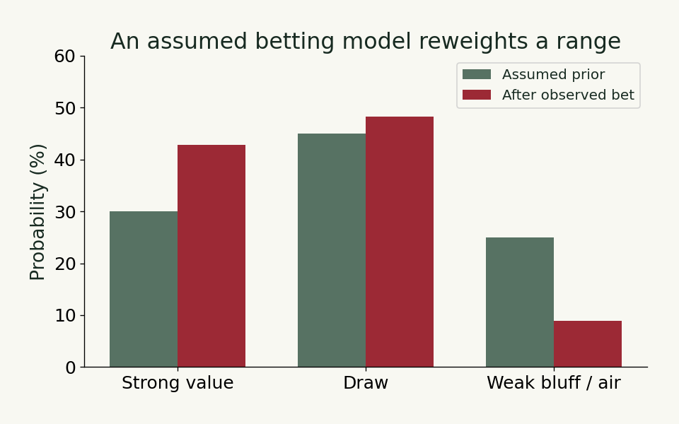
The bet raises the value probability from 30% to 42.86% and lowers pure air from 25% to 8.93%. Yet these posteriors are only as defensible as the likelihoods. If the player has been seen making the relevant bet only four times, estimating , , and with high confidence would be unjustified.
This is precisely why “he always has it when he uses that size” is poor statistical language. A small sample can alter a prior, but it rarely warrants a degenerate posterior of 0% or 100%.
The range-update process can be represented as:
The deeper lesson is that a blocker is not merely a solver vocabulary term. It changes the denominator of Bayesian inference. Behavioral evidence should be applied after impossible combinations have been removed.
Expected value, bluffing, and strategic response
Probability becomes strategically meaningful when attached to consequences. For a choice among actions , expected value is
where indexes future states and is the payoff associated with reaching state after choosing .
A fold can conventionally be assigned incremental at the current node because already invested chips are sunk. That does not mean folding the entire hand was costless from the beginning.
Calls and pot odds
Let:
- = pot after the opponent's bet but before Hero's call,
- = Hero's call,
- = Hero's showdown equity if no further betting occurs.
Hero gains net when winning and loses when losing, so
The break-even equity is therefore
Stating how is defined is essential. Confusion frequently arises because some poker discussions call the pot before the opponent's bet , while others mean the pot currently displayed after the bet.
Worked example: river bluff-catch. The pot is 100 bb before Villain bets 75 bb. Thus bb, and Hero must call .
Suppose Hero loses to 18 value combinations and beats 8 bluff combinations, all equally weighted:
Then
The call is barely profitable under the model. Changing only one bluff combination changes the decision materially. Range uncertainty is therefore strategically more important than calculating to two decimal places.
Worked example: turn draw against an all-in. Suppose the pot is 80 bb and Villain shoves a final 20 bb. Hero has a genuinely clean nine-out draw with one card to come.
After Villain's bet, , , so
With 46 unseen turn-to-river cards,
Assuming every out wins, every miss loses, there is no rake, and no further action is possible,
The conclusion disappears if some “outs” are dirty.
Fold equity and bluffing
A pure bluff risking to win an existing pot , with zero equity if called, has
where is fold probability.
Setting EV to zero gives
Worked example: bluffing 40 into 60.
If Villain folds 45%, the bluff is profitable under the zero-equity terminal model:
But real bluffs may retain equity when called, and future streets may exist. Thus this is a building block, not a complete no-limit solution.
Equilibrium bluff ratios and defense
Consider a deliberately simplified river game with a perfectly polarized bettor: every value hand always beats the bluff-catcher and every bluff always loses if called. Let pot exist before a bet .
For a bluff to be indifferent between betting and giving up, the defender's call frequency satisfies
so
This is the familiar minimum-defense-frequency expression for this toy model.
For the defender to be indifferent to calling, let be the fraction of the bettor's betting range that is bluff:
hence
The corresponding bluff-to-value ratio is
| Bet as fraction of pot | Toy-model defense frequency | Bluff fraction of betting range | Bluff:value ratio |
|---|---|---|---|
| 1/3 pot | 75.00% | 20.00% | 1:4 |
| 1/2 pot | 66.67% | 25.00% | 1:3 |
| 3/4 pot | 57.14% | 30.00% | 3:7 |
| 1 pot | 50.00% | 33.33% | 1:2 |
| 1.25 pot | 44.44% | 35.71% | 5:9 |
| 1.5 pot | 40.00% | 37.50% | 3:5 |
| 2 pot | 33.33% | 40.00% | 2:3 |
These equations are often overgeneralized. They assume one remaining decision, no raises, no rake, no blocker-sensitive bluff-catcher differences, zero bluff equity when called, and a polarized betting strategy. Modern equilibrium computation handles far richer game trees, which is one reason CFR and related methods became so influential in poker. (Zinkevich et al. 2007; Lanctot et al. 2009)
Mixed strategies arise because deterministic choices can make an opponent's counterstrategy too profitable. In two-player zero-sum games, no-regret procedures such as CFR can converge toward equilibrium strategies under suitable conditions. (Zinkevich et al. 2007) This does not imply that a human should mechanically randomize at equilibrium frequencies against every opponent. If credible evidence indicates that an opponent overfolds, the best response can contain substantially more bluffs. The statistical problem is determining whether the apparent overfolding is real and stable enough to justify that deviation.
Value betting and weighted responses
A value bet should be evaluated against the range that calls, raises, and folds, not against the opponent's entire starting range.
Worked example: weighted calling range. Suppose an 80 bb pot reaches the river. Hero considers betting 40 bb. Villain has 24 equally weighted combinations:
- 4 better hands, calling 100%;
- 8 worse hands, calling 75%;
- 12 weaker unpaired holdings, calling 0%.
Weighted calls:
Thus Villain calls and folds 58.33%. Conditional on a call, Hero wins against 6 of the 10 effective combinations:
If Villain folds, Hero wins the existing 80 bb. If called and Hero wins, the net gain from the node is bb; if Hero loses, the loss is the 40 bb bet.
If checking leads immediately to showdown, Hero beats 20 of the 24 original combinations:
The bet adds 3.33 bb in the toy model. Notice that “Hero has 83.3% equity against the range” was not sufficient to calculate the bet's value. Response frequencies were needed.
Why naive multi-street pot odds fail
Worked example: the price of not realizing river equity. On a flop, Hero has nine clean flush outs. The pot is 60 bb; Villain bets 30. A common but incorrect argument says:
and Hero is receiving a 25% immediate pot-odds threshold, so calling must be profitable.
Suppose instead the model specifies:
- after Hero calls, the pot is 120;
- if the turn hits one of nine outs, Hero wins the current 90 bb that was available before calling, with no further money;
- if the turn misses, Villain makes a turn bet that forces Hero to fold.
The relevant one-street probability is , and
The “34.97% by the river” figure assumed access to both cards for the price of one call. Poker does not guarantee that.
Implied odds, reverse implied odds, position, future fold equity, and future strategic responses are therefore not cosmetic corrections to pot odds. They determine the value of the decision tree.
Rake and costs
Rake alters the amount actually available to win, and therefore changes break-even thresholds and equilibrium incentives. A fixed-pot equation should use the net contestable pot after applicable rake, not a fictional gross amount. Because rake schedules may be percentage-based, capped, stake-specific, format-specific, and platform-specific, a universally valid single “rake adjustment” does not exist.
The same principle applies to opportunity costs. In a cash game, the incremental EV of folding at a current decision can be set to zero even though time spent in a poor game, table-selection decisions, and bankroll capital have economic value. Those broader costs belong to a different decision level.
Variance and evidence of skill
A poker result is a random variable. Its expected value is
and variance is
The standard deviation is . When outcomes across periods are dependent,
That covariance term matters. Poker hands may be approximately independent with respect to card shuffles, but realized profits can still exhibit dependence through table composition, tilt, changing stack depth, opponent adaptation, session selection, stake changes, and common strategic conditions.
The law of large numbers does not say that a modest sample must resemble expectation. It says that, under appropriate assumptions, the sample average converges toward the expectation as sample size grows. The central limit theorem similarly requires conditions that should not be casually equated with “I played many hands.”
How much precision does a sample buy?
Poker databases commonly express cash-game outcomes in big blinds per 100 hands. Suppose, only for illustration, that independent stationary 100-hand blocks have standard deviation
For hands, there are such blocks, giving
An approximate 95% normal interval has half-width .
| Hands | SE, bb/100 | Approximate 95% half-width |
|---|---|---|
| 1,000 | 28.46 | ±55.78 |
| 10,000 | 9.00 | ±17.64 |
| 100,000 | 2.85 | ±5.58 |
| 1,000,000 | 0.90 | ±1.76 |
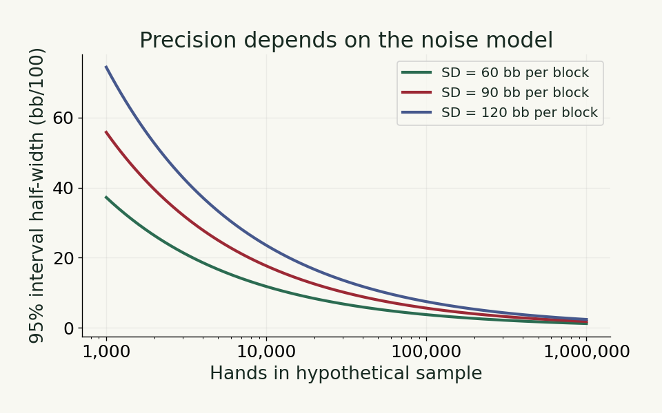
Worked example: what 100,000 hands can and cannot establish. If a player observed +4 bb/100 over 100,000 hands under this hypothetical model, an approximate interval would be
or roughly
That interval includes zero. The conclusion is not that the player is “probably losing.” It is that the assumed noise level leaves substantial uncertainty.
At the same , changing the assumed block standard deviation changes the 95% half-width:
| Hypothetical SD | 95% half-width |
|---|---|
| 60 bb/100 | ±3.72 |
| 90 bb/100 | ±5.58 |
| 120 bb/100 | ±7.44 |
This is why sample size cannot be discussed independently of variance.
Under this simplified known-variance model, planning for a 95% interval half-width of 3 bb/100 requires
Precision and power answer different questions. At that planning width, a two-sided 5% test has only about 50% power against a true +3 bb/100 mean: random estimates still fall on either side of the rejection boundary. Approximately 80% power requires about 706,400 hands, using the normal approximation and the same assumed variance. Neither figure is a universal sample-size requirement for a poker player.
Real datasets violate the ideal model in several directions. Opponents change, the player learns, game quality changes, rake differs, and hands within sessions need not be exchangeable. Historical win rate estimates an average over a historical environment, not an eternal player parameter.
Potter van Loon and colleagues illustrate both the promise and danger of population evidence. Their dataset contained 76.9 million hands and 456.1 million player-hand observations from more than 600,000 accounts at selected stakes over a 12-month period. (Potter van Loon et al. 2015) Their simulations suggested that, under their particular ranking and sampling framework, skill predominated over chance after roughly 1,500 hands. But the authors themselves stressed that the estimate depended on the method, did not account for possible serial dependence, and was affected by selection. It should not be transformed into the false statement “1,500 hands proves you are a winning player.” (Potter van Loon et al. 2015)
Levitt and Miles found that an a priori identified skilled group in the 2010 WSOP generated average ROI above 30%, compared with approximately -15% for the others. That is evidence that skill matters at the group level under their design, not a formula for tournament bankrolls or personal ROI precision. (Levitt & Miles 2014)
Statistical evaluation of poker skill
A frequentist confidence interval describes the long-run coverage properties of an inferential procedure under its assumptions. It does not mean “there is a 95% probability that this fixed true win rate lies in this realized interval.”
A Bayesian credible interval can be interpreted probabilistically about the parameter conditional on a model and prior, for example
That interpretation is more direct, but it purchases its meaning with explicit prior and likelihood assumptions.
Hypothesis testing introduces two familiar error modes:
- Type I error: concluding that an edge exists when the null model is true.
- Type II error: failing to detect a real edge.
Power depends on effect size, variance, sample size, test design, and significance threshold. Statistical significance is not the same as strategic importance. A reliably estimated +0.05 bb/100 effect may be economically negligible after costs.
Several poker-specific practices inflate false confidence:
Repeated checking. A player who examines a conventional fixed-sample -value after every few thousand hands and stops as soon as does not preserve the nominal false-positive rate. Sequential-analysis methods, always-valid -values, confidence sequences, or a prespecified stopping rule are safer. Work on always-valid inference explicitly addresses continuous monitoring and optional stopping. (Johari et al. 2021/2022)
Multiple comparisons. Searching dozens of stakes, positions, hand classes, filters, bet sizes, and date ranges until one subgroup “proves” a leak or edge invites false discoveries.
Data leakage. Building a strategy on a dataset and evaluating the strategy on the same observations rewards overfitting. Forward time splits, holdout periods, or genuinely prospective evaluation are more informative.
Regression to the mean. Players selected because they had an unusually hot period are likely, even with unchanged underlying skill, to look less extreme later.
Survivorship bias. Databases overrepresent players who continue playing. Potter van Loon et al. explicitly discussed selection and the possibility that weaker players disproportionately leave. (Potter van Loon et al. 2015)
Historical winning therefore establishes only the descriptive fact that realized past returns were positive. Inferring that future decisions have positive expectation additionally requires assumptions about persistence of skill, opponents, rules, rake, strategy, game selection, and measurement quality.
Opponent frequencies need denominators
A HUD statistic is a binomial-like proportion only after the opportunity set has been defined. Definitions vary somewhat by software, so the denominator should always be stated.
| Statistic | Typical numerator | Relevant denominator |
|---|---|---|
| VPIP | Hands voluntarily entering the pot preflop | Eligible hands dealt, under the tracker's convention |
| PFR | Hands with a preflop raise | Eligible hands dealt |
| 3-bet | Preflop reraises | Opportunities to reraise after facing a raise |
| Fold to 3-bet | Folds after facing a preflop 3-bet | Times player faces a 3-bet in the relevant role |
| Flop c-bet | Flop bets by last preflop aggressor | Eligible flop continuation-bet opportunities |
| Fold to flop c-bet | Folds facing a flop continuation bet | Eligible times facing one |
| Aggression frequency | Aggressive postflop actions | Defined action opportunities, tracker-specific |
| Showdown statistic | Showdown outcome or participation | Relevant reached-showdown or reached-river population |
“Villain folds to 3-bets 70%” is almost meaningless without knowing whether the denominator is 10, 100, or 10,000 comparable opportunities.
Worked example: shrinkage. Suppose an opponent has 3-bet 3 times in 12 opportunities:
A 95% Wilson interval is approximately
That is extremely wide.
Now suppose, solely for illustration, a population model is encoded as
whose prior mean is 20% with prior effective sample size 30. After observing 3 successes and 9 failures,
The posterior mean becomes
with an equal-tailed 95% credible interval of approximately 10.6% to 34.9%.
The raw 25% estimate has been partially pooled toward the prior population rate. This is shrinkage. It is useful because noisy extremes tend to be exaggerated, but the answer depends on the prior. A hierarchical model can estimate population and individual effects together rather than arbitrarily fixing a Beta prior. Multilevel modeling formalizes this partial-pooling principle. (Gelman 2007) For small binomial samples, naive Wald intervals also have well-known coverage weaknesses, motivating alternatives such as Wilson-style intervals. (Agresti 1998)
A mature opponent model should often condition further on position, stack depth, bet size, game format, opponent class, and previous actions. But every additional conditioning variable reduces sample size. This creates a fundamental bias-variance trade-off: aggregate statistics have more observations but less situational relevance; highly specific statistics may be relevant but hopelessly noisy.
Platform rules and ethics
Tracking rules are not universal. As of the currently published 2026 GGPoker Security & Ecology Policy, GGPoker prohibits real-time external assistance, prohibits mining other players' hand histories, and expressly lists HUDs, solvers, charts, and similar gameplay-influencing tools among prohibited auxiliary tools during play. (GGPoker policy 2026)
PokerStars' published third-party-tool guidance permits in-game HUD statistics based only on information accumulated through one's own play, while prohibiting certain advanced range, equity, ICM, and Nash-equilibrium tools while the client is open. (PokerStars policy) Americas Cardroom currently states that hand trackers and HUDs may use statistics based solely on a player's own collected hand history, with current-hand information excluded, while real-time advice tools are prohibited. (ACR policy)
These policies can change. Statistical capability does not imply permission to use the capability during live play.
Calculators, simulations and solvers
An equity calculator answers a probability question under supplied cards and ranges. If all legal runouts are enumerated, its result may be exact conditional on those inputs.
For a practical application with current source boundaries, the multiway guide distinguishes a nearby three-way study from the actual four- or five-way live hand.
A Monte Carlo calculator samples runouts or hands rather than enumerating all of them. If independent simulations estimate a Bernoulli event with probability ,
A solver addresses a different problem. It approximates strategies in a game model, often using regret minimization, decomposition, abstraction, value functions, or search. CFR minimizes counterfactual regret, and in two-player zero-sum extensive-form settings its average strategy has equilibrium-convergence guarantees. MCCFR replaces full traversals with sampled portions of the tree, lowering iteration cost while introducing estimator variance. (Zinkevich et al. 2007; Lanctot et al. 2009)
DeepStack combined recursive reasoning, decomposition, and a learned value function; it defeated professional HUNL players over tens of thousands of hands. (Moravčík et al. 2017) Libratus used a large blueprint strategy, nested subgame solving, and self-improvement and defeated four elite HUNL specialists over 120,000 hands. (Brown & Sandholm 2018) Pluribus extended superhuman performance to six-player no-limit hold'em using self-play and search, while the authors explicitly emphasized that multiplayer games do not inherit all of the strong theoretical properties of two-player zero-sum equilibrium computation. (Brown & Sandholm 2019)
AIVAT demonstrates another statistical point: better estimators can reduce evaluation variance without changing the agent's actual playing strength. Burch and colleagues reported an 85% reduction in standard deviation in a poker human-machine evaluation setting. (Burch et al. 2018) Thus “play more hands” is not the only statistical response to noisy performance. Better experimental design and variance reduction can also improve inference.
Worked computational experiment: Monte Carlo versus exact probability. For a nine-out flop draw:
A simulation was actually conducted for this article using NumPy 2.3.5, default_rng(seed=20261014), with 1,000,000 hypergeometric two-card draws from 9 desired and 38 undesired cards.
Result:
Estimated Monte Carlo standard error:
Approximate 95% simulation interval:
The exact value lies comfortably inside. The Monte Carlo estimate differs from the exact value by about 0.031 percentage points.
The exercise illustrates four different notions that poker discussions frequently conflate:
- Simulation precision: how much sampling noise remains.
- Solver convergence: how close an iterative strategy is to its game-model target.
- Model validity: whether the cards, ranges, sizes, abstractions, rake, and rules represent the real game.
- Strategic validity: whether the modeled opponent behavior is relevant to the human actually being played.
A solver can be numerically precise and strategically misapplied at the same time.
Tournament chips and prize equity
Cash games and tournaments have different objective functions. In a cash game without external utility complications, a chip won is generally worth the same monetary amount as another chip of the same denomination. In a tournament, chips are claims on uncertain future prizes and cannot normally be cashed at face value. This creates nonlinear monetary equity.
Independent Chip Model
The Independent Chip Model assigns probabilities of finishing positions recursively from stack shares. Its mathematical structure is closely related to sequential finish-order probability models such as Harville's 1973 work. Harville derived finish-order probabilities from relative strengths and evaluated the model on 335 horse races. (Harville 1973) Poker's ICM application should therefore be understood as a probabilistic model, not a theorem that tournament chips literally behave according to its assumptions.
For stacks , ICM begins with
Conditional on player finishing first, the probability that finishes second is recomputed from the remaining stacks. Prize equity is then the expected payout over finish positions.
Worked example: positive chip EV, negative monetary EV. Three players have stacks
and prizes
monetary units.
Exact ICM recursion yields:
| Player stack | ICM monetary equity |
|---|---|
| 50 | 38.393 |
| 30 | 32.750 |
| 20 | 28.857 |
Hero has 30 chips. The 50-chip leader shoves, effectively risking Hero's entire 30. If Hero folds, ICM equity remains 32.75.
If Hero calls and wins, stacks become
giving Hero ICM equity of 41.
If Hero loses, Hero finishes third and receives 20.
Let be Hero's probability of winning the all-in. Monetary EV of calling is
Calling breaks even against folding when
so
By contrast, the all-in is chip-EV positive whenever .
If , Hero's chip change is
chips in expectation, but monetary equity is
which is 1.20 monetary units below folding.
That gap is a simple expression of tournament risk premium.
This example treats the listed stacks as the decision-state alternatives, with no blinds, dead money, ties or other branches. ICM omits future positional advantage, differences in player skill, blind pressure, strategic leverage, bounty structures and individual utility. Its answer is exact for the stated recursive model, but that model is an approximation to tournament play.
Tournament ROI is correspondingly difficult to estimate. Returns are highly skewed because rare final tables and wins produce a large fraction of long-run profit. Cashing percentage can stabilize while ROI remains imprecise. Two players with identical cash rates can have radically different payout distributions. “I have a 20% cash rate” therefore says little about profitability unless field size, payouts, buy-ins, and finish distribution are known.
Bankroll models and their limits
Bankroll management is not an exercise in finding a universal number of buy-ins. Required reserves depend on edge, variance, game format, correlation, stake flexibility, withdrawal behavior, and acceptable ruin probability.
Classical ruin theory studies the probability of reaching a lower absorbing boundary under stochastic gains and losses; Ferguson's work is one early formal contribution to optimal betting under ruin constraints. (Ferguson 1965) Kelly's 1956 paper established a connection between proportional wagering and long-run logarithmic growth under known favorable probabilities. (Kelly 1956) Poker only imperfectly matches that framework because a player cannot freely scale every edge, the edge itself is estimated, games change, and one player's bet size changes opponent behavior.
Define a hypothetical continuous bankroll process , where is standard Brownian motion and time is measured in 100-hand blocks. For fixed positive drift, the eventual probability of touching zero is exact inside this model:
Here B is the starting balance in big blinds, μ is the expected change in big blinds per block, and σ is the standard deviation of a one-block increment in big blinds. For zero or negative drift, the eventual hitting probability is 1 in this ideal infinite-horizon process. The positive-drift formula follows from the Brownian hitting result in Lawler, Example 5.2.2; applying continuous diffusion to actual poker is an approximation.
Assume purely hypothetically:
| True mean | Bankroll | Brownian approximate ruin probability |
|---|---|---|
| 3 bb/100 | 2,000 bb | 22.73% |
| 3 bb/100 | 3,000 bb | 10.84% |
| 3 bb/100 | 5,000 bb | 2.46% |
| 5 bb/100 | 2,000 bb | 8.47% |
| 5 bb/100 | 3,000 bb | 2.46% |
| 5 bb/100 | 5,000 bb | 0.21% |
Worked example: estimation risk matters more than the decimal. At a presumed +5 bb/100 edge and 3,000 bb bankroll, the approximation gives about 2.46% ruin risk. If the true edge is only +3 bb/100, the same bankroll produces about 10.84%.
Thus a bankroll policy based on an overestimated edge can be dramatically less conservative than intended. The table itself should not be used as a bankroll prescription. The Brownian model assumes fixed stakes, stationary positive drift, continuous diffusion, no withdrawals, no behavioral errors, and play continuing until ruin. Real poker violates all of these assumptions.
A prudent bankroll framework should therefore distinguish:
- mathematical volatility, driven by game outcomes;
- parameter uncertainty, especially uncertainty about the true edge;
- structural uncertainty, such as future game quality or rake;
- behavioral risk, including tilt, poor game selection, or stake escalation;
- personal utility, because psychological or financial tolerance for drawdowns differs.
Judge the decision before the result
Statistical literacy has emotional as well as mathematical value because poker produces many events that feel more informative than they are.
Tversky and Kahneman's classic work documented systematic judgment errors arising from representativeness, availability, and insufficient attention to base rates. (Tversky 1974; Tversky 1973) Their earlier work on belief in the “law of small numbers” described people's tendency to expect small samples to resemble the population too closely. (Tversky 1971) Nickerson's review documented the broad literature on confirmation bias, while Baron and Hershey demonstrated outcome bias, in which decision quality is judged partly by information that was unavailable when the decision was made. (Nickerson 1998; Baron 1988)
Poker supplies a natural setting for each:
| Misinterpretation | Statistical correction |
|---|---|
| “I have missed eight flush draws, so the next one is due.” | Under a fair shuffle, earlier misses do not make the next relevant unseen card more likely. |
| “I won five sessions, so my strategy is proven.” | Results are noisy observations; evaluate uncertainty and decision quality. |
| “Every time he overbets he has the nuts.” | Count relevant opportunities, use a prior, and estimate uncertainty. |
| “My river call was bad because I lost.” | Judge the action using probabilities and information available before the result. |
| “The solver says 73%, so betting 73% must be objectively correct.” | The precision is conditional on the solver's model, ranges, abstraction, and equilibrium target. |
| “That player is running hot, so he is likely to keep winning.” | Separate genuine persistent skill/state effects from random streak interpretation. |
The “hot hand” literature deserves special caution. Gilovich, Vallone, and Tversky's influential basketball study argued that people perceived serial dependence beyond what the data supported. Later, Miller and Sanjurjo identified a finite-sample bias in common analyses of streak shooting and reported evidence favoring a hot-hand effect after correction. (Gilovich 1985; Miller 2018) The scholarly lesson is broader than whether one basketball dataset contained a hot hand: intuitions about streaks are unreliable, but statistical tests themselves can also be biased if their conditioning structure is misunderstood.
In poker, the emotionally healthy version of statistical reasoning is not “variance means nothing matters.” It is “a single outcome contains less information about decision quality than the decision process that generated it.”
A repeatable decision process
A rigorous poker decision can be organized as the following loop:
This framework has ten practical steps:
Observe. Record cards, position, effective stack, pot, previous actions, legal bet sizes, tournament state, and relevant opponent information.
Define unknowns. Opponent holding, future cards, fold frequencies, bet frequencies, future actions, and possibly utility or tournament monetary value.
Condition the state space. Remove impossible combinations before applying strategic assumptions.
Construct a prior range. Use position, earlier actions, population information, and player-specific evidence.
Update after actions. Treat actions as evidence whose likelihood differs by hidden hand class.
Calculate conditional equity. Evaluate hand versus the posterior distribution, not versus a convenient single hand.
Model available actions. Include folds, calls, sizes, raises, and future branches.
Compute expected objective. In cash games this may approximate chip EV after rake; in tournaments it may require monetary-equity or utility considerations.
Stress-test assumptions. Identify which uncertain parameter can reverse the preferred action.
Learn. Update range and behavioral models after observing showdowns and future actions, while avoiding overreaction to tiny samples.
A complete case: what changes the river call?
Consider a six-max cash game, blinds 0.5/1 bb, with 150 bb effective stacks. Rake is omitted solely to keep the arithmetic transparent.
Hero is on the button with
Hero opens to 2.5 bb. The small blind folds. The big blind 3-bets to 11 bb. Hero calls.
The pot is
This case study does not claim that calling rather than 4-betting is equilibrium optimal. Preflop equilibrium depends on rake, stack depth, raise sizes, range assumptions, and game model. The call is treated as the observed starting point.
Flop:
Big Blind bets 7.5 into 22.5. Hero calls.
The pot becomes
Hero has the nut-flush draw plus two overcards, but “two overcards plus nine flush outs” should not be converted into a naive 15-out count. An ace or king can be dirty against sets, two pair, or stronger made hands; some flush cards can alter full-house possibilities on later paired boards.
For the later turn-call calculation, stipulate Big Blind’s range after observing the turn bet on a blank :
This is a transparent teaching model, not a solver prescription.
Turn:
Big Blind bets 25 into 37.5. The pot before Hero's call is therefore
Hero must call 25. Both players have 131.5 bb behind before this turn bet: 150 − 11 − 7.5. After the big blind bets 25, that player has 106.5 bb; Hero still has 131.5 until calling.
If betting stopped after the call and all river equity were perfectly realized, the break-even equity would be
The exact enumeration performed earlier gives Hero 41.136% showdown equity against the stipulated range.
That establishes one fact:
Under the specified range, Hero has substantially more than the 28.57% equity required in a hypothetical terminal-showdown version of the decision.
It does not mathematically prove that calling is best. There are 131.5 bb behind before the turn bet, future river betting matters, a raise may have fold equity, and the opponent's range itself is uncertain.
Hero calls. The pot becomes
Both players now have 106.5 bb. If the later 65 bb river bet is called, each has 41.5 bb remaining. The final pot is 217.5 bb: 108.5 from each player and 0.5 from the folded small blind. The stack and pot ledger therefore reconcile at every street.
River:
Hero now has top pair with ace kicker. Big Blind bets 65 into 87.5.
After the bet,
The call threshold is
Now apply card removal again. The removes one KJs combination. Under the turn range, the effective river masses can be grouped as:
- strong value: sets plus KJs, effective mass ;
- worse one-pair hands AJs and QJs, mass ;
- weaker unpaired holdings T9s, 98s, QTs and AQs, mass . These include weaker unpaired holdings and high-card hands; not every surviving suit combination had a live draw on the turn.
Suppose the river bet likelihoods are modeled as:
These are assumptions, not observed truths.
Betting masses become
for hands beating Hero,
for worse pairs, and
for bets from weaker unpaired holdings.
There are no ties among the legal holdings in this stipulated river range. Hero's posterior equity when calling is therefore
Set this equal to the required 29.885%:
Solving gives
That parameter is the decision boundary.
If weaker unpaired holdings bet 35% of the time:
and
If they bluff 50%:
and
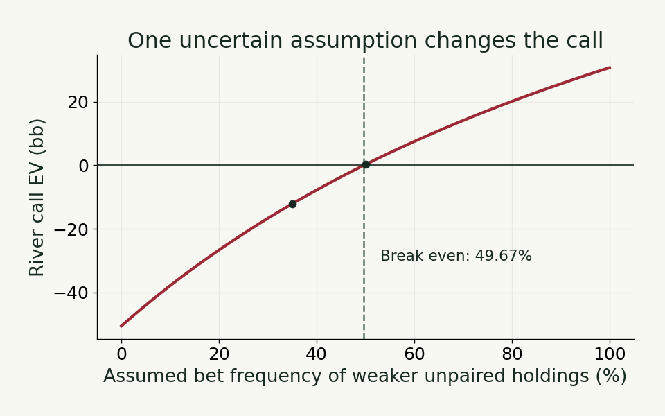
A modest change in one uncertain behavioral likelihood flips the recommendation.
That is the core statistical lesson of the entire article. The difficult question is not whether 29.885% has been calculated correctly. It has. The difficult question is whether is closer to 35% or 50%, whether the range omitted important value combinations such as AA or other Kx holdings, whether earlier action likelihoods were modeled correctly, and whether this particular opponent's behavior is stationary enough for historical data to apply.
What survives a change in assumptions?
Precision is not the same as relevance. A million-run equity simulation can estimate the equity of the wrong range to four decimal places. Numerically eliminating Monte Carlo error does not eliminate model misspecification.
Blockers and Bayes are one process. Blocker analysis is best understood as prior conditioning. Known cards remove impossible hidden states; action evidence then reweights the surviving states. Treating blockers and “range reads” as unrelated techniques obscures their mathematical unity.
Variance creates a learning problem, not merely a bankroll problem. High variance does more than produce downswings. It corrupts feedback. If players judge strategic changes from short-term profit, noisy outcomes can reward bad modifications and punish good ones. Decision-level review, controlled comparisons, and large-sample evaluation can be more informative than a graph of cumulative winnings.
Solver precision can generate false epistemic confidence. Modern poker AI established that formidable strategies can emerge from equilibrium-oriented computation and search. DeepStack, Libratus, and Pluribus are genuine scientific milestones. (Moravčík et al. 2017; Brown & Sandholm 2018; Brown & Sandholm 2019) But the strongest scientific interpretation is conditional: they demonstrate the power of formal game models, not that a commercially displayed frequency is an immutable law of human poker. A solver's tiny numerical error can coexist with large input-range error.
The objective function matters. Chip EV, cash-game monetary EV, tournament monetary equity, log-growth objectives, and individual utility can recommend different actions. The ICM example showed mathematically how a +chip-EV call can be -monetary-EV.
Inference is not intervention. Observing that a strategy characteristic correlates with profitable players does not prove that forcing another player to adopt it will produce the same gain. Confounding by skill, table selection, stakes, opponent quality, and correlated strategic choices remains possible. Potter van Loon et al. found persistence and associations with playing style, but observational analysis cannot automatically identify causal strategy improvements. (Potter van Loon et al. 2015)
Actionable recommendations
For players and coaches, the highest-value statistical habits are not memorizing more percentages. They are:
- Maintain range weights in combinations, not hand labels.
- Separate equity against a model from confidence in the model.
- Report every opponent percentage with its opportunity count.
- Prefer regularized estimates to raw extreme frequencies when samples are small.
- Analyze multi-street EV as a tree instead of applying “by the river” equity to a one-street price.
- Track strategy changes prospectively, preferably with prespecified evaluation windows or sequential methods.
- Conduct sensitivity analysis whenever a recommendation depends on uncertain bluff, fold, or value frequencies.
- Keep solver study offline and comply with current platform rules. (GGPoker policy 2026; PokerStars policy; ACR policy)
- Treat bankroll recommendations as risk models with assumptions, not universal commandments.
- Review decisions using information available at the time, not the card that happened to arrive.
Use conditional conclusions
The intellectual error that most often undermines quantitative poker analysis is asking a precise mathematical tool to answer a question it was not designed to answer.
Combinatorics can tell us exactly how many combinations survive card removal. It cannot tell us how frequently a human chooses each action.
Bayes' theorem can coherently update beliefs once priors and action likelihoods are supplied. It cannot guarantee that those likelihoods were estimated from a relevant population.
An equity calculator can exactly evaluate a stipulated range. It cannot certify the range.
Expected value can identify the best action inside a decision model. It cannot prove that the modeled future responses are correct.
A confidence interval can quantify sampling uncertainty under assumptions. It cannot turn a changing poker ecosystem into a stationary experiment.
A solver can approximate equilibrium inside a formal game. It cannot guarantee that the real opponent follows the modeled strategy or that the abstraction is strategically adequate.
ICM can transform stacks into a coherent approximation of tournament prize equity. It cannot represent every future strategic advantage.
Bankroll theory can quantify risk conditional on drift and variance. It cannot remove uncertainty about the drift itself.
The strongest poker reasoning therefore consists of disciplined conditional statements: given these cards, this weighted range, these behavioral likelihoods, these future-response assumptions, this objective function, and this uncertainty model, action A has higher expected value than action B.
That sentence is less psychologically satisfying than “the solver says call,” but it is scientifically stronger.
Poker expertise at its quantitative best is thus not the possession of more probabilities. It is the ability to distinguish what is known exactly, what is estimated from data, what is assumed strategically, what remains uncertain, and which conclusions survive reasonable changes in those assumptions.
Reproduce the calculations
The Python reproduction script enumerates the weighted range and river outcomes, checks the pot and stack ledger, and reproduces the Bayes, ICM, sample-size and Brownian examples using the standard library. Run it with Python 3.12. To repeat the recorded one-million-run simulation, install NumPy 2.3.5 and use python poker-under-uncertainty-reproduce.py --monte-carlo. The seed is 20261014. Other NumPy versions may produce different samples.
The calculation results in JSON record the exact fractions, assumed inputs, Python and NumPy versions, seed, simulation result and its sampling interval. They document a computation, not evidence that the toy range describes any real opponent.
A useful review asks two separate questions: does the arithmetic follow from the inputs, and what evidence supports those inputs? Reproducing the first does not settle the second. No reader study has yet established how beginners understand or use this essay or the surrounding lessons.
Sources and editorial note
This article was adapted with AI assistance from a supplied research draft. The publication revision corrected the stack ledger, clarified range labels and model assumptions, replaced temporary research citations with traceable references, and reran the numerical examples. Source studies retain their own methods and limitations. Operator policies were checked on October 14, 2026; consult the linked current policy before using any software during play.
Agresti, A., & Coull, B. A. (1998). Approximate is better than “exact” for interval estimation of binomial proportions. The American Statistician, 52(2), 119-126. DOI. The paper motivates interval procedures with better coverage than the naive Wald interval.
Baron, J., & Hershey, J. C. (1988). Outcome bias in decision evaluation. Journal of Personality and Social Psychology, 54(4), 569-579. DOI.
Bowling, M., Burch, N., Johanson, M., & Tammelin, O. (2015). Heads-up limit hold'em poker is solved. Science, 347(6218), 145-149. DOI. The work established the “essentially solved” result for heads-up limit hold'em under its formal criterion.
Brown, N., & Sandholm, T. (2018). Superhuman AI for heads-up no-limit poker: Libratus beats top professionals. Science, 359(6374), 418-424. DOI. Author abstract.
Brown, N., & Sandholm, T. (2019). Superhuman AI for multiplayer poker. Science, 365(6456), 885-890. DOI. Author supplement.
Burch, N., Schmid, M., Moravčík, M., Morrill, D., & Bowling, M. (2018). AIVAT: A new variance reduction technique for agent evaluation in imperfect information games. Proceedings of the AAAI Conference on Artificial Intelligence, 32(1). DOI.
Ferguson, T. S. (1965). Betting systems which minimize the probability of ruin. Journal of the Society for Industrial and Applied Mathematics, 13(3), 795–818. DOI.
Gilovich, T., Vallone, R., & Tversky, A. (1985). The hot hand in basketball: On the misperception of random sequences. Cognitive Psychology, 17, 295-314. Publisher.
Harville, D. A. (1973). Assigning probabilities to the outcomes of multi-entry competitions. Journal of the American Statistical Association, 68(342), 312-316. JSTOR/DOI.
Harsanyi, J. C. (1967). Games with incomplete information played by “Bayesian” players, Part I: The basic model. Management Science, 14(3), 159-182. DOI.
Harsanyi, J. C. (1968). Games with incomplete information played by “Bayesian” players, Part II: Bayesian equilibrium points. Management Science, 14(5), 320-334. DOI.
Johari, R., Koomen, P., Pekelis, L., & Walsh, D. (2021 online; 2022 issue). Always Valid Inference: Continuous Monitoring of A/B Tests. Operations Research, 70(3), 1806–1821. Published paper. Sequential inference methodology, not a poker trial.
Kelly, J. L., Jr. (1956). A new interpretation of information rate. Bell System Technical Journal, 35, 917-926. DOI.
Lanctot, M., Waugh, K., Zinkevich, M., & Bowling, M. (2009). Monte Carlo sampling for regret minimization in extensive games. Advances in Neural Information Processing Systems 22. Primary paper.
Levitt, S. D., & Miles, T. J. (2014). The role of skill versus luck in poker: Evidence from the World Series of Poker. Journal of Sports Economics, 15(1), 31-44. DOI.
Miller, J. B., & Sanjurjo, A. (2018). Surprised by the hot hand fallacy? A truth in the law of small numbers. Econometrica, 86(6), 2019-2047. DOI.
Moravčík, M., Schmid, M., Burch, N., Lisý, V., Morrill, D., Bard, N., Davis, T., Waugh, K., Johanson, M., & Bowling, M. (2017). DeepStack: Expert-level artificial intelligence in heads-up no-limit poker. Science, 356(6337), 508-513. DOI; arXiv.
Nickerson, R. S. (1998). Confirmation bias: A ubiquitous phenomenon in many guises. Review of General Psychology, 2(2), 175-220. DOI.
Potter van Loon, R. J. D., van den Assem, M. J., & van Dolder, D. (2015). Beyond chance? The persistence of performance in online poker. PLOS ONE, 10(3), e0115479. DOI.
Tversky, A., & Kahneman, D. (1971). Belief in the law of small numbers. Psychological Bulletin. DOI.
Tversky, A., & Kahneman, D. (1973). Availability: A heuristic for judging frequency and probability. Cognitive Psychology, 5, 207-232. DOI.
Tversky, A., & Kahneman, D. (1974). Judgment under uncertainty: Heuristics and biases. Science, 185(4157), 1124-1131. DOI.
Zinkevich, M., Johanson, M., Bowling, M., & Piccione, C. (2007). Regret minimization in games with incomplete information. Advances in Neural Information Processing Systems 20. Primary paper.
Gelman, A., & Hill, J. (2007). Data Analysis Using Regression and Multilevel/Hierarchical Models. Cambridge University Press. DOI.
GGPoker. (2026). Security & Ecology Policy, current version displayed as 20260313. The policy restricts real-time assistance, mining, HUDs, solvers, charts, and related auxiliary tools during gameplay. Official policy.
PokerStars. Third-party tools policy guidance. Its published guidance permits restricted own-history HUD use while the client is open but prohibits advanced range/equity/ICM/Nash tools in that state. Official policy.
Americas Cardroom. Security and third-party-tool policies. Its current policy allows own-history numerical HUDs subject to restrictions while prohibiting real-time advisory software. Official policy.
Lawler, G. Stochastic Calculus: An Introduction with Applications, Example 5.2.2, printed p. 152. Author manuscript. The Brownian hitting formula used here requires a fixed drift and variance.
Continue with the research map, results in context or a practical hand review. The site’s decision-quality essay develops the same habit of judging choices using the information available at the time.